
Research note · metric scale from inertial data
Can a 360° camera measure its own scale?
Our 360° reconstructions get their metric scale from a smartphone carried alongside the camera. We replaced it with the accelerometer and gyroscope already inside the camera. The short answer: against a LiDAR scanner riding on the same pole, the camera's own IMU gets scale right to 0.81% on average over nine surveys — 2.4× closer than the phone it replaces. The longer answer is the trap on the way: the textbook alignment, solved over a whole survey, overestimates scale by 3.4% with a consistent sign. Solving each stretch of the walk on its own and averaging removes the bias, and on fifty production surveys (33 km) the method ran unattended, passed its own checks every time and agreed with the phone to σ = 2.3%.
01The question
Every metric model we make borrows its scale from a phone
Structure-from-motion recovers the shape of a scene and the path of the camera, but not their size: without a known length somewhere, the whole model is only defined up to a similarity transform [2]. Our pipeline supplies that length with a second device. During the walk the operator takes a short burst of smartphone photos, whose poses come from ARKit or ARCore and are metric; the photos are registered into the 360° model and their scale is transferred to it.
It works, but it has three costs. It is a second device and a second procedure. It makes the metric reference heterogeneous, because two AR platforms and their versions do not behave alike. And it extrapolates: the burst takes about fifteen seconds over a few metres, so the scale of a walk of several hundred metres rests on a small corner of it. Measured against a co-mounted LiDAR (§02), the phone reference is off by 1.9% on average and by up to 4.4% on a single survey.
The camera already carries a better candidate. The Insta360 X5 and X6 record a gyroscope and an accelerometer at 1 kHz into the video file. The accelerometer measures specific force in metres per second squared, and for a trajectory in arbitrary model units there is exactly one scale factor at which its second derivative matches the measured accelerations once gravity is accounted for. Finding that factor is the classic visual-inertial initialisation problem [3–5]; the question is whether it holds up offline, on minutes-long surveys, from a consumer camera.
Three numbers hold the story together; the rest of the note reconstructs them one at a time.
02The gain
Against a LiDAR on the same pole, the IMU is 2.4× closer than the phone
The decisive test needs a reference that measures metres directly and shares nothing with either candidate. We carried a 3DMakerPro Eagle LiDAR scanner [6] on the same pole as an Insta360 X5 through nine surveys of 98 to 245 m, one from a first campaign and eight from a second. For each survey the LiDAR cloud was registered to the reconstruction with a closed-form initialisation and a scaled ICP cascade on the dense clouds [8,9]; the factor it returns is the error of the phone reference that scaled the model, and comparing it with the IMU estimate gives the IMU's error. All nine surveys are public [25]: recording, IMU, reconstruction, LiDAR cloud and the registration between them, so every number in this section can be checked from the raw data.
The inertial scale has a mean error of +0.07%, a mean absolute error of 0.81% and a worst case of 2.11%. The phone reference, on the same models, has a mean of −0.41%, a mean absolute error of 1.94% and a worst case of 4.36%. Neither shows a systematic sign — both behave like unbiased references — but the IMU is the closer of the two on seven surveys of nine.
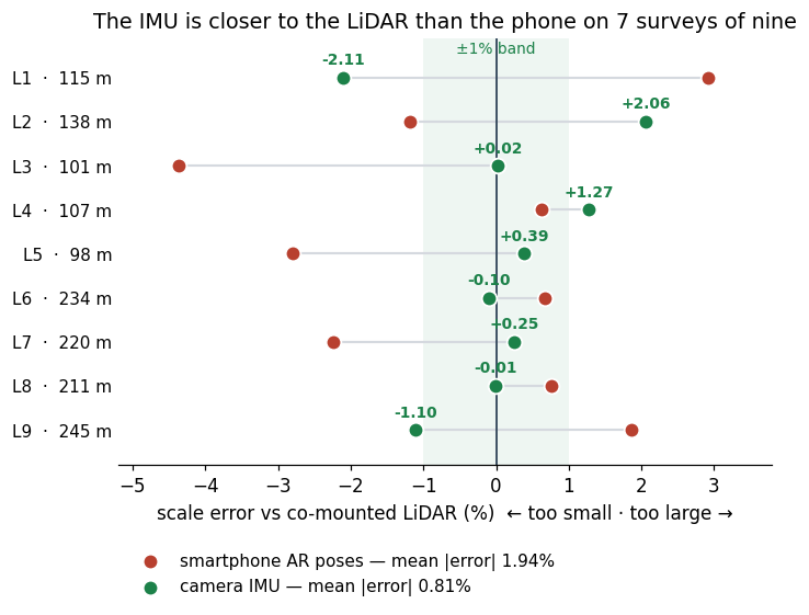
| Scale error vs LiDAR, 9 surveys | mean | mean |error| | worst | closer on |
|---|---|---|---|---|
| smartphone AR poses (anchors the model) | −0.41% | 1.94% | 4.36% | 2 of 9 |
| camera IMU, segment-wise (this note) | +0.07% | 0.81% | 2.11% | 7 of 9 |
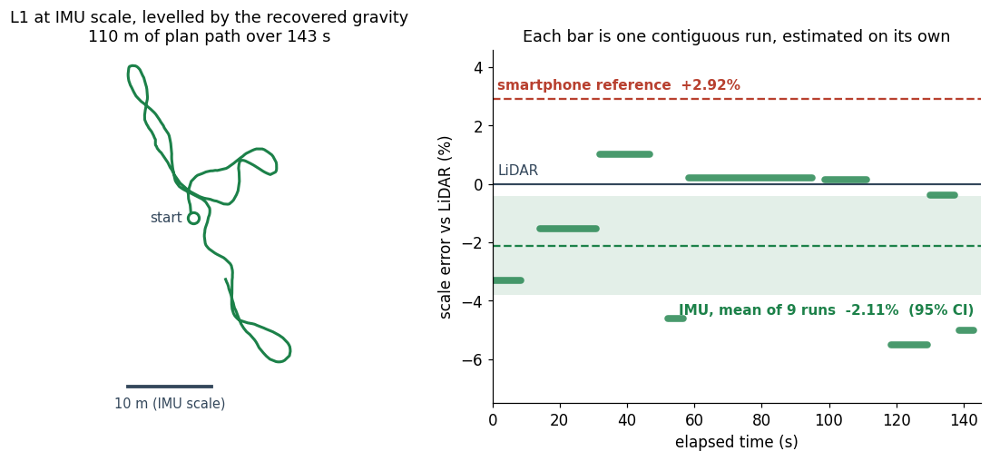
Survey L1, shown below, is the hardest of the nine for the IMU, and even there the camera's own sensor lands closer to the LiDAR than the phone does (−2.11% against +2.92%). Across all nine, an instrument that shares nothing with the LiDAR agrees with it to 0.8% on average; the phone, measured the same way, is off by 1.9%.
03A risk we had to defuse
The sensor is good enough; the clock model is what can break it
Before trusting a single number we characterised the sensor as it lands in the file. The X6 gyroscope is flat white noise above 100 Hz at about 0.006 °/s/√Hz, the level of a good consumer MEMS part; the X5 stores values its firmware has already low-pass filtered. We checked synchronisation without a calibration target by estimating the camera's rotation from the video alone (tracked corners, a fisheye model and a pure-rotation fit [10–12]) and correlating it with the gyroscope: on a hand-held sequence spinning at up to 480 °/s the correlation is 0.99 on all three axes and peaks at 0 ms. The IMU timestamps in the file are already on the video clock, to within about ±5 ms. An eleven-minute recording on a table gave the accelerometer's gain: a mean specific force of 9.8092 m/s² against a local gravity of 9.806, correct to 0.03%.
What can break the method is the other half of the time model: when, on the IMU clock, each reconstruction frame was taken. Frames are sampled at a fixed nominal interval, and the nominal value is not good enough. An error of 0.1% slips the video against the IMU by 0.4 s over a ten-minute survey — more than a frame interval — and the scale comes out wrong by tens of percent. A local optimiser started from the nominal value rescues it only on smooth motion; on brisk walking it stays put, the hand-eye residual sits at 3–4° per interval, and the survey fails.
So both timing constants are estimated from the data: a coarse grid over the interval, a fine grid of ±0.4% around the best candidate with the offset re-centred, then a small simplex, all minimising the angular disagreement between the SfM rotations and the integrated gyroscope [13]. With the right interval the residual is 0.05–0.18° per interval on every survey in this note, and the recovered camera-to-IMU rotation is the same across independent surveys, as it must be for a rigid body. A wrong interval is also detectable without ground truth: re-estimate the time offset on the first and last quarter of the survey, and the two disagree by a drift proportional to the error — below 10 ms on our surveys, 530 ms with the nominal interval on a ten-minute one. Above 60 ms the estimator refuses to answer.
04The cost
The textbook alignment is biased high by 3.4%, on nine surveys of ten
With clocks settled, the scale comes from a linear system. Between consecutive frames the accelerometer is integrated at 1 kHz in the model frame, starting from the SfM orientation and propagated by the gyroscope [14,15]. Each interval then gives a position and a velocity equation that are linear in the scale s, the gravity vector g, the accelerometer bias b and one velocity per frame:
s·(Ck+1 − Ck) − vkΔt − ½gΔt² + Jkb = Δpk
vk+1 − vk − gΔt + Kkb = Δvk
The standard formulation solves all of it at once, with g and b shared across the survey — they are, after all, properties of the survey rather than of a stretch of it. Measured against the ten surveys with an external reference (the nine LiDAR ones and a marker survey), that formulation overestimates scale by 3.39% on average, with the same sign on nine of the ten. When we first ran it on the eight LiDAR surveys of the second campaign, the IMU came out high on all eight: precise, repeatable and wrong.
We first suspected the sensor, and we checked. The accelerometer gain is right to 0.03%, and the static recording measures the bias drift directly: it moves like a thermal warm-up, by 0.042 m/s² over ten and a half minutes, about 0.013 over a three-minute survey — an order of magnitude too little to produce a 3% shift. The argument we kept is structural. Gravity enters every position equation as ½gΔt², a term the same size as the displacement itself, so any way in which the effective gravity direction is not constant over minutes — for instance a slow residual orientation drift in the reconstruction — is absorbed by the one parameter left free to absorb it, the scale. The joint solution is not an average of the per-stretch solutions and is not even constrained to lie among them. We have not isolated the exact mechanism; the experiments that follow show where the cure is.
05Countermeasures
Stop sharing gravity and bias, and the bias goes — however you cut the survey
If shared nuisance parameters are the problem, the cure is to estimate them locally. The names in the table below sound alike, so it helps to be precise about what they have in common and what they do not. Every construction uses the same frames, the same IMU samples and the same two equations per interval. Every one of them also respects the survey's natural breaks: the reconstruction discards blurry frames, which cuts the walk into contiguous runs of frames no more than 1.2 s apart, and a velocity can only be chained inside a run, never across a gap. What changes between the rows is a single thing: how many independent linear systems the survey is solved as, and therefore how many frames share one scale, one gravity vector and one accelerometer bias.
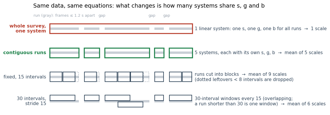
Whole survey, one system is the textbook formulation of §04. It keeps the runs apart for the velocities but puts every run into one least-squares problem that has a single unknown scale, gravity and bias. There is one answer, and the runs recorded minutes apart are forced to agree on where «down» is. Contiguous runs looks almost the same on a diagram: it has the same boxes around the same data. But each run is now its own problem with its own scale, gravity and bias, and the result is the mean of the per-run scales. The difference is the whole point. Whatever makes the effective gravity wander over minutes is soaked up by each run's own g, which it can afford to spend. In the joint system it can only be soaked up by s. The joint scale is also not an average of the run scales. It is the scale of one compromise fit, and nothing keeps it inside their range.
The other rows answer the obvious follow-up: are the natural runs special, or would any split do? Fixed windows cut each run into consecutive blocks of N intervals. Sliding windows take every block of N intervals at stride one, so each interval is counted many times. The stride variant sits in between, with 30-interval windows every 15. Every block is solved alone, as in contiguous runs, and the block scales are averaged. We compared them all on the ten surveys with ground truth.
| Construction | Systems per survey | Outcome (10 surveys) |
|---|---|---|
| whole survey, one system | 1 — s, g, b shared by all runs | mean +3.39%, |err| 3.43%, worst 6.05% — rejected |
| fixed, 15 intervals | many short blocks inside each run | mean −0.54%, |err| 1.39% — biased low helps |
| sliding, 60 intervals | long overlapping windows, step 1 | mean +0.86%, |err| 1.17%, worst 4.56% — biased high helps |
| fixed, 25 / 30 / 50 intervals | blocks of fixed length inside each run | mean −0.44 / −0.32 / −0.24%, |err| 0.95 / 0.90 / 0.90% — works |
| 30 intervals, stride 15 | overlapping windows, step 15 | mean −0.20%, |err| 0.89% — works |
| contiguous runs | 1 per run — the survey's own breaks, no length to tune | mean −0.05%, |err| 0.85%, worst 2.11% — adopted |
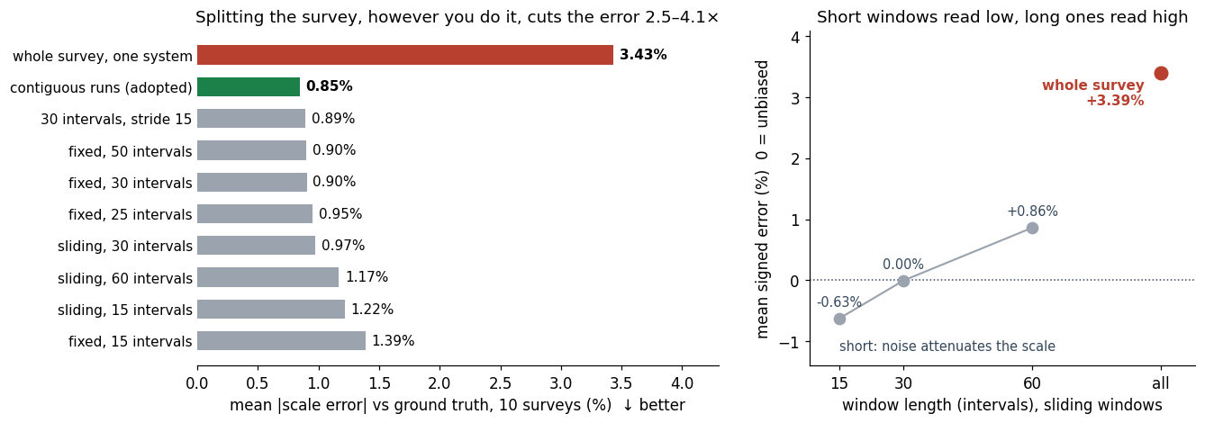
Every windowed variant beats the joint system, by a factor between 2.5 and 4.1: the gain comes from not sharing gravity and bias, not from any clever segmentation. Across all constructions the error ranges only from 0.85% to 1.39%, and overlap barely matters — sliding windows at stride one produce five to fifteen times more estimates and move the error by less than two tenths of a point. The survey's own runs come out best, if only by a few hundredths, and they are the one construction with no length to choose.
06The winning lever
Two biases of opposite sign bound the estimate, and the survey's own runs sit between
The right panel above is the whole mechanism. Short windows are biased low: noise in the SfM camera centres enters the position equation as an error in the regressor, which attenuates the fitted scale — −0.6% for sliding windows of 15 intervals, zero at 30. Long windows are biased high, because they start sharing gravity over minutes again — +0.9% at 60 — and the whole survey is the extreme case. The contiguous runs the reconstruction already produces — maximal stretches of frames no more than 1.2 s apart, broken wherever blurry frames were discarded — are 15 to 60 intervals long, right where both effects vanish. That is why we adopted them over a tuned fixed length: they reach the same accuracy with no knob to set.
The one case they cannot handle is a recording with no gaps. With nothing discarded, the whole walk is a single run, and a single run is the joint system of §04. The estimator therefore keeps the runs as they are whenever they are enough for a mean, and only when fewer than four usable runs remain does it cut them into windows of about 25 intervals. That fallback reads about half a percent low in the ablation, so it is a safety net, not the method: on none of the sixty surveys in this note does it fire.
Solving per run also makes the estimate self-auditing. Every run must recover a gravity magnitude between 9.3 and 10.3 m/s² — the scale does not need it, a correct alignment cannot miss it — or it is dropped. The spread of the per-run scales, 1–3% within a survey, gives the uncertainty of their mean directly (0.3–1.5% over five to thirteen runs). A survey fails if that uncertainty exceeds 2.5%, if fewer than four runs survive, if its two halves disagree by more than 6%, or if the clock drift test of §03 trips. On one recording whose reconstruction jumps by 19 m mid-walk, the estimator reports failure rather than a scale.
One lesson from building these checks: a quality gate inherits the biases of the estimate it reads. Our first version read gravity, spread and the half-versus-half test off the joint solution, and turned away good surveys whenever that solution collapsed — L5, accurate to 0.39%, among them. The checks now read the runs, and the joint solution survives only as a diagnostic.
07From study to deployment
Fifty production surveys, 33 km, no failures — and no ground truth
The same estimator, with the same settings, was then run on fifty production surveys, 246 to 708 s and 193 to 1,261 m each, which we have released as OverMaps360-50 [16]. All fifty produce an estimate that passes every check. The conditioning matches the surveys with ground truth: median uncertainty on the mean 0.36%, median per-run spread 2.0%, median recovered gravity 9.79 m/s², median hand-eye residual 0.08°. Against the phone reference the IMU agrees to a standard deviation of 2.3%.
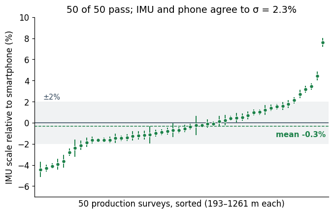
On average the IMU reads 0.3% below the phone (median −0.6%, 31 surveys of fifty below). The difference is uncorrelated with run length (r = −0.15), duration or path length, but it does move with the size of the phone anchor. On the 42 surveys whose photo burst spans less than 12 m the IMU is 0.8% lower; on the eight whose burst spans 16 to 29 m it is 2.4% higher, a figure one survey at +7.6% weighs on heavily.
Two honest footnotes. First, nothing on this set can say which of the two is right. The phone carries a measured error of 1.9% against the LiDAR and the IMU 0.8%, so a 0.3% mean difference is well inside what both allow, and the anchor-size trend could belong to either; a third, metric instrument on the same scenes is the only way to assign it, and we have not run one. Second, the set exercises the textbook alignment far beyond §04, and it confirms the verdict: the joint solution lies above the per-run mean on 34 surveys of fifty, and on three it collapses outright to scales between 0.000 and 0.064 while the per-run estimates on the same surveys stay tight.
A printed-marker survey closes the deployment picture. On a survey with ArUco markers [7], whose own geometry pins scale to 0.987–1.005 once a 1% print shrinkage is measured and corrected, the IMU reads 0.989 and the phone 1.000: both inside the target.
The estimator alone, on a public benchmark. Every survey so far mixes two sources of error: the estimator, and the reconstruction it reads. To isolate the first we ran it on the 30 sequences of the public Hilti-Trimble-Oxford benchmark [24]: indoor walks through a construction site, 69 to 276 s and 72 to 352 m each (5.5 km in total), recorded with an Insta360 ONE RS 1-inch and its 1 kHz IMU, with the camera trajectory measured by a rigidly attached LiDAR-inertial system. The estimator is handed that reference trajectory directly, decimated to 3 Hz and supplied as a model of poses only. The recovered scale has a mean error of −0.07% (median −0.24%) and a standard deviation of 1.28%; 18 sequences of 30 land within 1%, 28 within 2%, the worst at 3.2%, and all thirty pass the quality checks. On the 25 sequences the benchmark uses for ranking, the mean error is −0.26% and the mean absolute error 0.85%. On trajectories without reconstruction error the estimator has no bias, and its spread per sequence is about 1% on recordings of one to five minutes. The same runs also speak to §04: on these trajectories even the whole-survey solution is unbiased (−0.06% on average), which supports the reading that its 3.4% on our surveys comes from slow inconsistencies of the reconstruction, not from the sensor.
The thirty trajectories double as a test that the estimator is blind to the frame it is handed. Each was supplied at scale 1/40, 1 and 40, with a random rotation and translation: once divided by the applied factor, the three recovered scales agree on every sequence to better than 0.0001%, and all pass. Any units, any orientation.
08The alternative we rejected
Monocular metric depth cannot be the reference at this accuracy
The tempting shortcut needs no inertial data at all: modern networks predict metric depth from a single image [17–20], so the ratio between predicted depth and the SfM depth of the sparse points should give the scale. We tested it with MoGe-2 and MoGe-3, rectifying fisheye frames to 90° pinhole views with the known field of view. On L1, over all 290 frames, MoGe-2 is off by −3.2% and MoGe-3 by −18.8% against the LiDAR. Within a frame the prediction is proportional to the SfM depth to about 1%: the networks get the shape right and the size wrong.
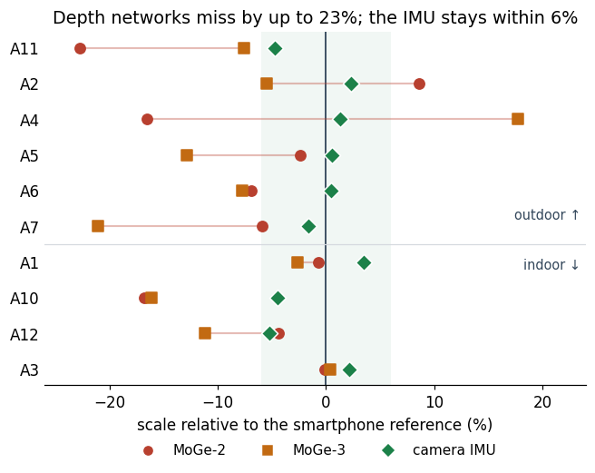
We expected outdoor scenes to be the problem, and they are worse on average (mean |bias| 11–12% outdoors against 5–8% indoors), but the split is not clean: two indoor surveys come back within 3% from both networks and a third is off by 16% with both. The two networks disagree with each other by up to 34% on the same scene, and the newer, larger one is not more accurate. What controls the error is how close a scene is to the training distribution, which no one can check at capture time. A depth network makes a fine coarse sanity check on the inertial scale; as a reference, its bias is larger than any disagreement it would be asked to settle.
09Why it matters
The metric reference moves inside the camera, and it audits itself
The practical result is that the smartphone step can leave the capture procedure. The scale now comes from a sensor that records every second of every walk, rather than from fifteen seconds of it at one spot; it is the same sensor on every capture instead of whatever phone the operator carries; and it arrives with its own evidence — recovered gravity, clock drift, hand-eye residual, per-run spread — that says when an estimate should not be trusted. On the surveys where an instrument reading metres exists, that estimate is within 0.81% on average and never worse than 2.1%.
The transferable lesson concerns the textbook method more than the camera. Linear visual-inertial initialisation was designed for the first seconds of a live tracker; run in batch over minutes, its shared-nuisance assumption quietly converts any slow inconsistency into scale. A batch user who trusts the closed form over the whole sequence gets a result that is precise, repeatable and 3% wrong — exactly the kind of error that only an outside instrument exposes.
Methods note
Protocol. Poses come unchanged from the production reconstruction (dual-fisheye rig SfM in the COLMAP family [2]); no model was rebuilt for this study. IMU data are read from the native recording at 1 kHz [1]. Timing: interval and offset estimated per survey by a two-stage grid plus simplex on the gyroscope-vs-SfM rotation residual, camera-IMU rotation by Kabsch [13]. Scale: linear alignment over preintegrated intervals [14,15], solved per contiguous run (frames ≤ 1.2 s apart, ≥ 8 intervals, per-run |g| in 9.3–10.3 m/s²), outliers above five times the median residual removed before a second solve; the reported scale is the mean of the run scales. LiDAR references: closed-form initialisation plus scaled ICP of the scanner cloud to the reconstruction [8,9]; fiducial reference from triangulated ArUco centre distances within 50° of the optical axis. Benchmark: the 30 reference trajectories of [24], decimated to 3 Hz, scaled by 1/40, 1 and 40 with a random rotation and translation, and supplied as pose-only models; the error is the recovered scale times the applied factor, minus one.
Data rigor. Every number in this note was computed with the public estimator [23] at its default settings, on inputs anyone can obtain; the lens, the references and a no-exclusion rule were fixed before any result was read. The ten surveys with ground truth are the ones the method was developed on; the fifty production surveys with a usable phone reference are the independent check, and a new LiDAR campaign processed blind is the next step. Excluded and stated: one recording with 19 m discontinuities (the estimator reports failure), one bundle-adjustment experiment in non-metric units, two recordings without phone photos. Static sensor figures come from a third X5 unit; the MoGe comparison uses IMU values from the earlier whole-survey estimator (§08 caption). Survey identities are anonymised throughout.
Limits. The LiDAR is a consumer SLAM instrument; its per-point accuracy (2–5 cm at 10–40 m) does not limit a scale fit over millions of points. All surveys with ground truth were taken with the X5; the X6 is characterised as a sensor. The estimator reads one lens of the dual-fisheye rig, lens 1 throughout, fixed in advance; lens 0 gives 0.76% on the LiDAR set and passes all fifty production surveys, reading 0.6% lower on average. The 0.3% offset on the production set is unattributed. The linear solution is not yet followed by a non-linear refinement with gyroscope bias [21], which leaves room to improve on the closed form.
10Conclusions
What we take away
The IMU inside an Insta360 X5, combined with the poses the reconstruction already computes, gives metric scale with no smartphone: 0.81% mean absolute error against a co-mounted LiDAR over nine surveys, against 1.94% for the phone reference, inside the 1% tolerance of a printed marker target, and a 2.3% agreement with the phone over fifty unattended production surveys. It gets there only under two conditions — the frame timing is estimated from the data rather than taken at face value, and the alignment is solved per contiguous run rather than jointly, which takes the error against ground truth from 3.43% to 0.85%.
The recipe transfers to any camera that logs its IMU: check the IMU clock against video-only rotation before anything else; estimate the frame timing and keep a drift test that catches it when it is wrong; never share gravity and bias across minutes of data; let the spread of independent segments be the error bar; and read quality checks off the quantity you actually report.
—References
- Gyroflow. telemetry-parser — reads the IMU stream from the native Insta360 container (github.com/gyroflow/telemetry-parser).
- Schönberger & Frahm. Structure-from-Motion Revisited (COLMAP). CVPR 2016 — the SfM family of the reconstructions whose poses feed the estimator.
- Martinelli. Closed-Form Solution of Visual-Inertial Structure from Motion. IJCV 2014 — the linear relation the alignment solves.
- Mur-Artal & Tardós. Visual-Inertial Monocular SLAM with Map Reuse. RA-L 2017 — linear inertial initialisation in ORB-SLAM.
- Qin, Li & Shen. VINS-Mono: A Robust and Versatile Monocular Visual-Inertial State Estimator. T-RO 2018 — the same initialisation in a live tracker.
- 3DMakerPro. Eagle LiDAR scanner — the co-mounted metric reference of nine surveys; SLAM of the LOAM family [22].
- Garrido-Jurado et al. Automatic Generation and Detection of Highly Reliable Fiducial Markers under Occlusion (ArUco). Pattern Recognition 2014 — the printed marker reference.
- Umeyama. Least-Squares Estimation of Transformation Parameters Between Two Point Patterns. TPAMI 1991 — closed-form initialisation of the LiDAR registration.
- Besl & McKay. A Method for Registration of 3-D Shapes. TPAMI 1992; Rusinkiewicz & Levoy, Efficient Variants of the ICP Algorithm, 3DIM 2001 — the scaled ICP that reads the LiDAR scale.
- Shi & Tomasi. Good Features to Track. CVPR 1994; Bouguet, Pyramidal Lucas-Kanade Feature Tracker, 2001 — the video-only rotation estimate of the sync test.
- Kannala & Brandt. A Generic Camera Model and Calibration Method for Conventional, Wide-Angle, and Fish-Eye Lenses. TPAMI 2006 — the fisheye model.
- Fischler & Bolles. Random Sample Consensus. CACM 1981 — robust rotation fit in the sync test.
- Kabsch. A Solution for the Best Rotation to Relate Two Sets of Vectors. Acta Cryst. A 1976 — camera-IMU rotation from rotation vectors.
- Lupton & Sukkarieh. Visual-Inertial-Aided Navigation for High-Dynamic Motion in Built Environments Without Initial Conditions. T-RO 2012 — inertial preintegration.
- Forster et al. On-Manifold Preintegration for Real-Time Visual-Inertial Odometry. T-RO 2017 — the form of the preintegrated terms.
- OverTheReality. OverMaps360-50 — the fifty production surveys of §07 with embedded IMU and smartphone poses, Hugging Face 2026 (huggingface.co/datasets/OverTheReality/OverMaps360_50).
- Wang et al. MoGe: Unlocking Accurate Monocular Geometry Estimation for Open-Domain Images. 2024 — the metric-depth networks tested in §08 (MoGe-2, MoGe-3).
- Yin et al. Metric3D. ICCV 2023 — metric depth from a single image.
- Bhat et al. ZoeDepth. 2023 — metric depth from a single image.
- Yang et al. Depth Anything. CVPR 2024 — monocular depth foundation model.
- Campos, Montiel & Tardós. Inertial-Only Optimization for Visual-Inertial Initialization. ICRA 2020 — the non-linear refinement we do not yet run.
- Zhang & Singh. LOAM: Lidar Odometry and Mapping in Real-time. RSS 2014 — the SLAM family behind the LiDAR reference.
- OVER Research. imu-metric-scale — the estimator, sensor tools and ablation scripts used for every number in this note (github.com/OVR-Platform/imu-metric-scale).
- Centanni, Zhang, Tao, Kindle, Neuhaus, Koss, Patel, Helmberger, Szymanska, Graeber & Fallon. Hilti-Trimble-Oxford Dataset: 360 Visual-Inertial Benchmark with Floor Plan Priors for SLAM and Localization. arXiv:2607.06464, 2026 — the public benchmark whose 30 reference trajectories test the estimator on its own in §07.
- OverTheReality. Insta360 surveys with LiDAR reference for metric-scale validation — the nine LiDAR surveys of §02 with recordings, IMU, reconstructions, LiDAR clouds and registrations, Hugging Face 2026 (huggingface.co/datasets/OverTheReality/insta360-imu-metric-scale-surveys).