
Research note · reconstruction accuracy
How accurate is our automatic 360°-camera reconstruction pipeline?
We benchmarked our 360° photogrammetry pipeline against a LIDAR survey of the same site, captured simultaneously on a shared rig. The short answer: the reconstruction agrees with the LIDAR to a median of 3.9 cm — the reference scanner's own declared accuracy — with no accumulated drift over a 118 m path. The longer answer is the one disagreement we found, a uniform 2.9% scale offset, and the chain of measurements showing the reconstruction did not create it: the model copies its metric reference to 0.03%, the disagreement lies between that reference and the LIDAR, and the only tape measure on record sides with the model. Either way, it is one scalar away from disappearing.
01The question
«How accurate is it?» deserves a number, not an adjective
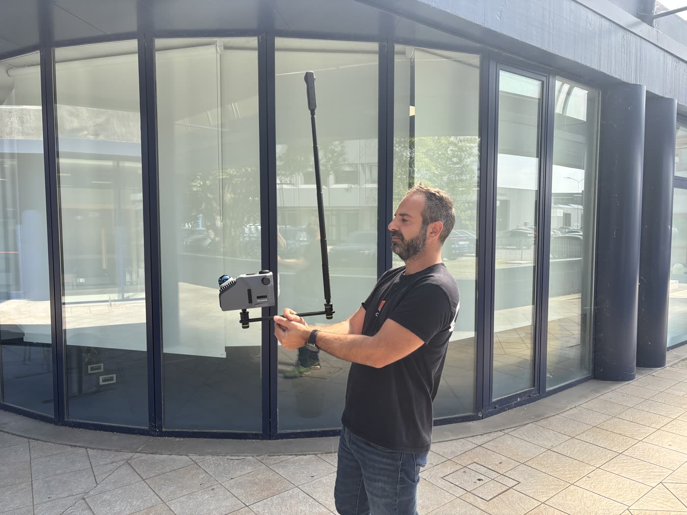
Our pipeline turns a ten-minute walk with a 360° camera into a dense, metric 3D model of a site. We say «survey-grade» in slides; this note is about earning that phrase. We put a LIDAR scanner on the same pole as the 360° camera, walked the site once, and built the two reconstructions by fully independent means — ours from imagery through structure-from-motion [1], the reference from LIDAR range measurements. Same walk, same light, two instruments that share no assumptions.
The capture is genuinely the thing we sell: one operator, one pass, no tripods, no targets. Below, the input stream and what the pipeline makes of it.
Three numbers hold the story together; the rest of the note reconstructs them one at a time.
02The result
Half the surface within 3.9 cm, three quarters within 10 cm
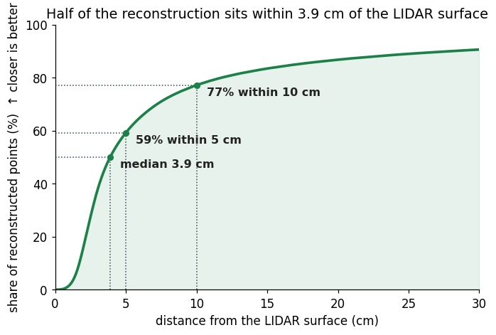
The headline protocol is deliberately blunt: downsample both clouds to a 5 cm voxel grid and measure, for each of the 1.07 million reconstructed points, the distance to the nearest LIDAR surface point. After the scale correction discussed below, the median is 3.9 cm; 59.5% of the surface is within 5 cm and 77.6% within 10 cm.
One calibration before the plot: the reference scanner itself has a manufacturer-declared accuracy of about 4 cm [6]. A median agreement of 3.9 cm therefore sits at the floor of what this reference can certify — at this level we are measuring the pair of instruments, and the reconstruction is not distinguishable from the reference's own error budget.
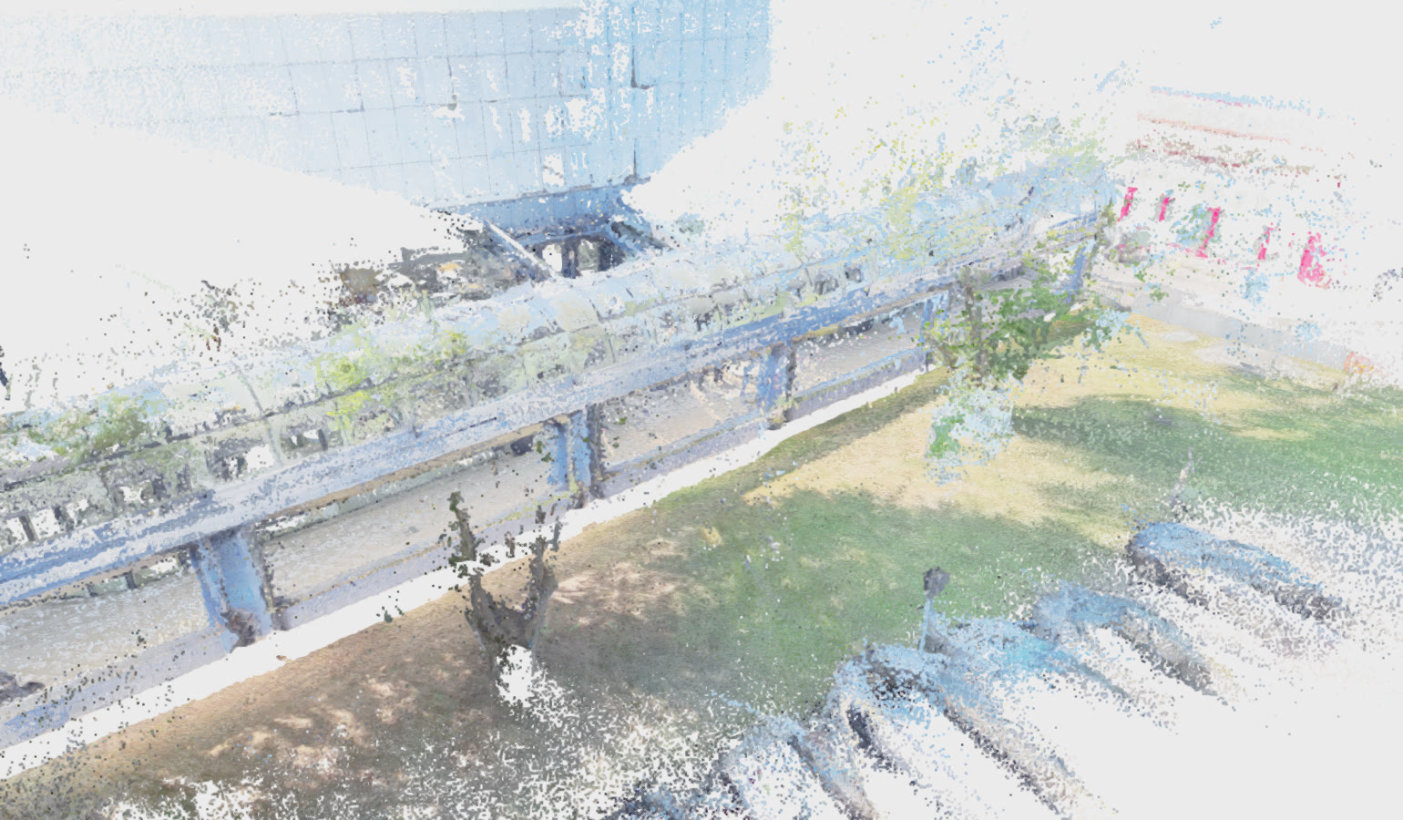
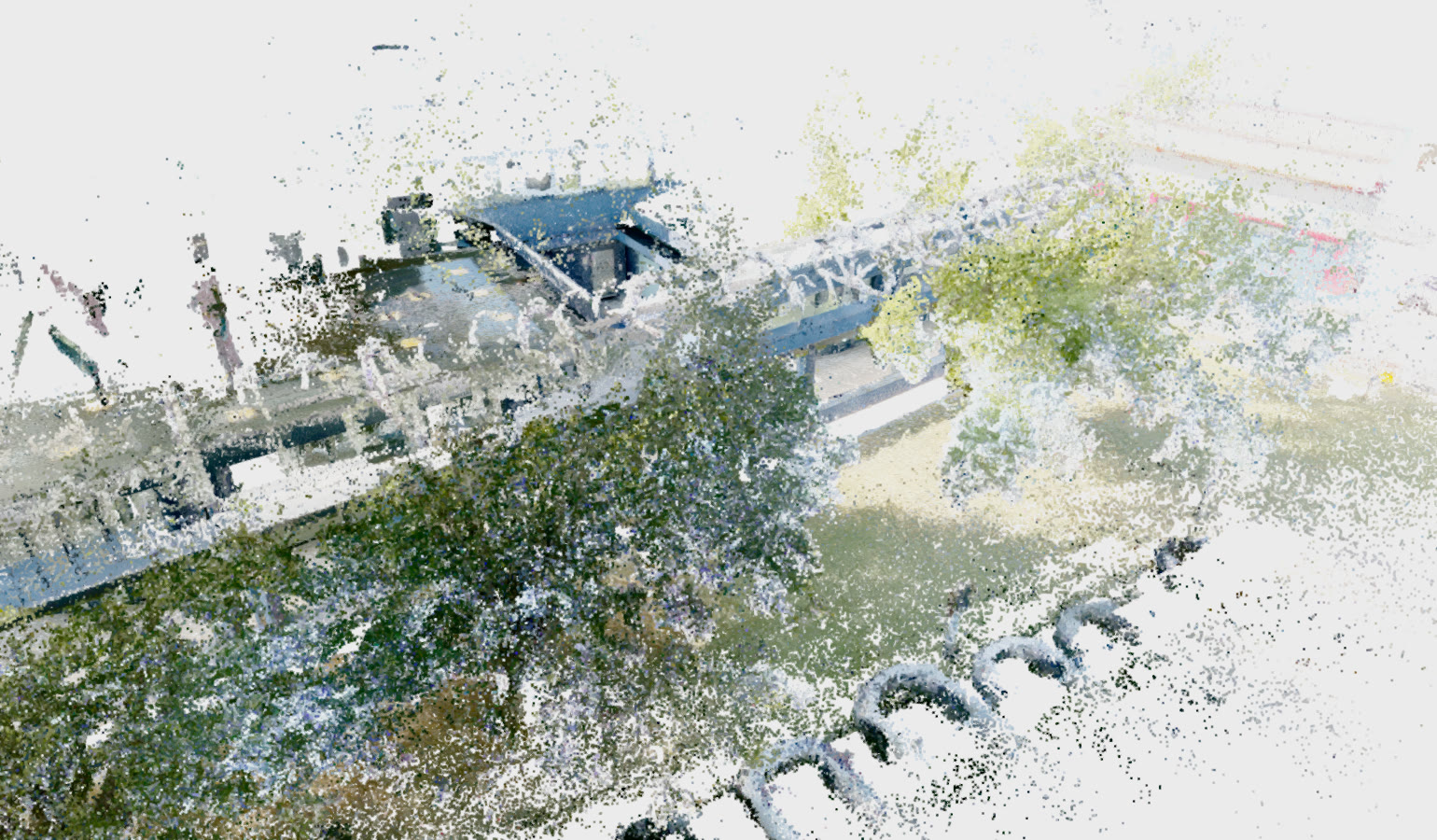
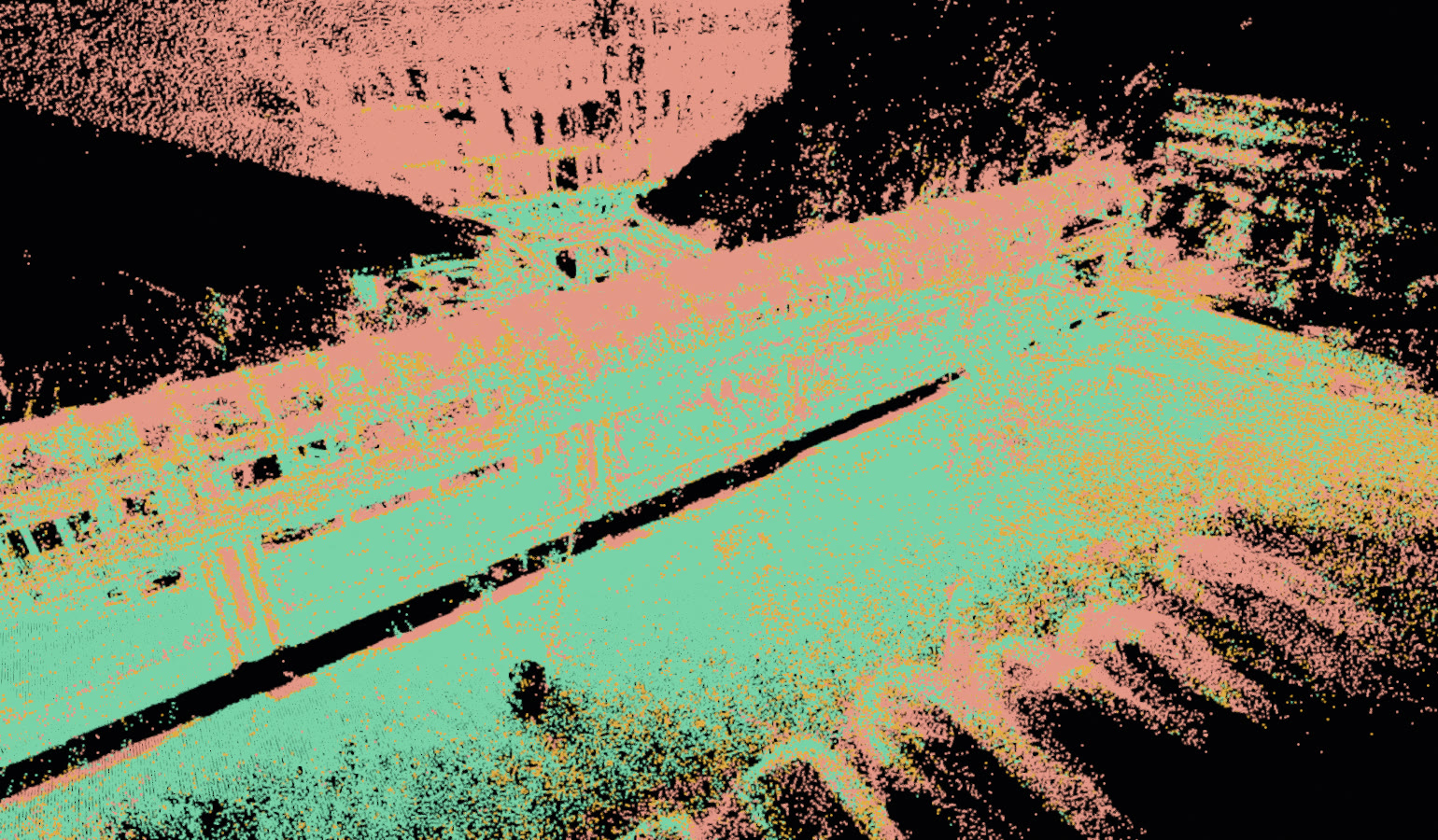
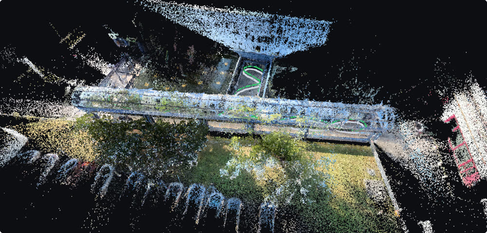
Numbers first, but geometry is easier to trust when you can look at it. Here is the same site as both instruments see it, from the same viewpoint:
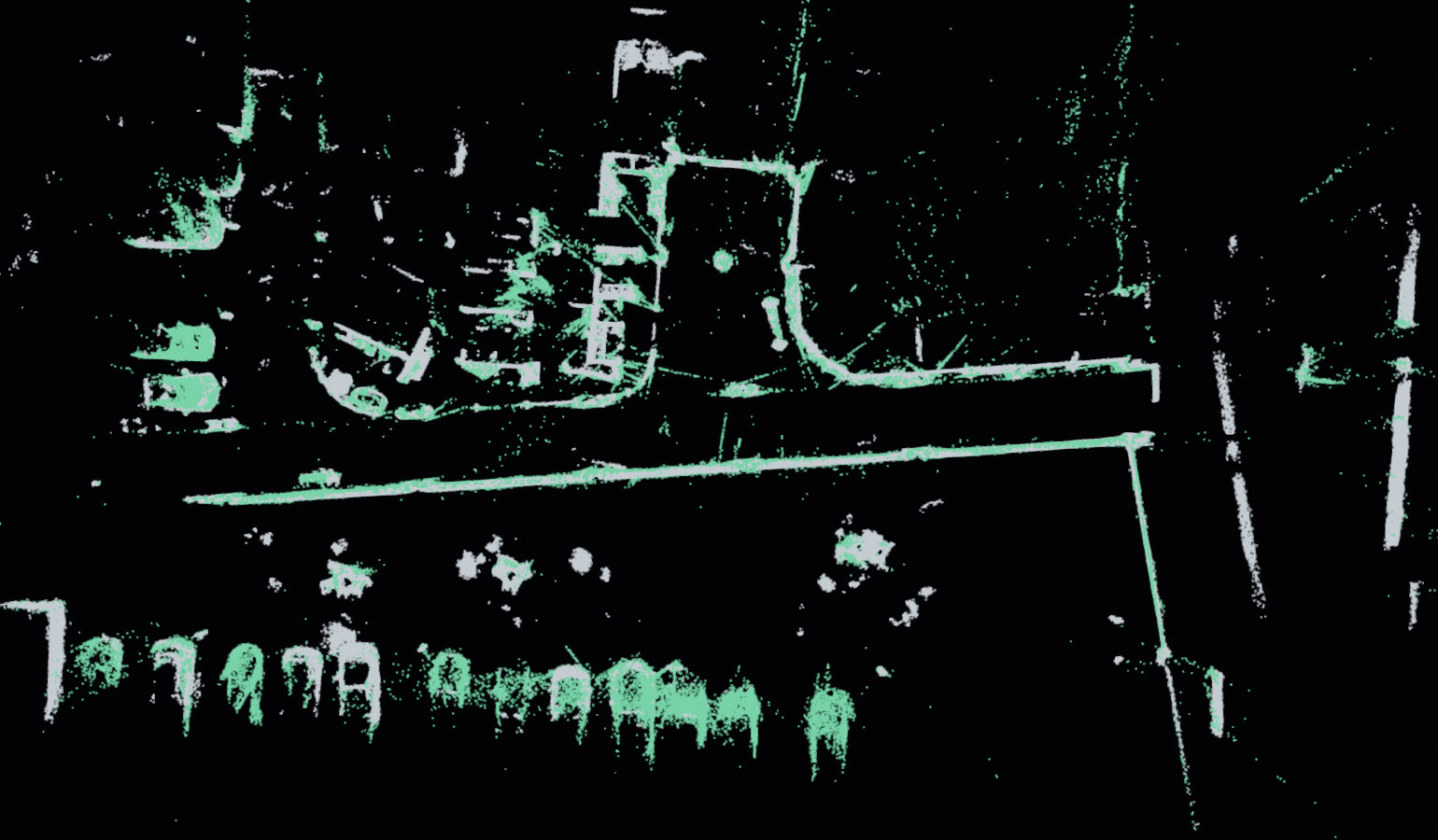
And because a claim like «the walls coincide» should be checkable, a 1 m horizontal slice of both clouds, seen from above — the classic floor-plan test. Where the alignment is good, green (ours) draws directly on top of gray (LIDAR):
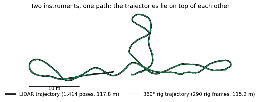
The camera path itself tells the same story. The pipeline registered 385 rig frames along 115 m; the LIDAR tracked 1,414 poses along 118 m. Aligned with the same transform as the clouds, the two paths agree to a median of 6.1 cm (p90 11.2 cm) over the whole loop [2]:
03A risk we had to defuse
The obvious alignment method quietly converges to a lie
Before any accuracy number exists, the two reconstructions must be aligned — and the alignment itself is the first place this comparison could have silently gone wrong. The obvious tool is free-scale ICP between the two camera trajectories. It is also degenerate: two smooth curves can be brought closer by shrinking one onto the other, so the optimizer happily trades scale for proximity and returns a spurious optimum. A curve, unlike a surface, does not constrain scale.
So the protocol splits the problem in two. First, a closed-form similarity transform (Umeyama [2]) over arc-length correspondences between the trajectories — searching across travel direction and trim, immune to the shrinking failure because it never iterates. Then the scale is refined where it is actually observable: scaled ICP on the dense surfaces [3], at four decreasing correspondence thresholds (50, 25, 12, 6 cm). The scale estimate moved by less than ±0.0003 across all four thresholds — the sign of a well-conditioned optimum, not a lucky one.
The trajectory-only estimate, for the record, landed at 2.49% — half a point off the surface-based consensus. That gap is the degeneracy talking, and it is why every scale number quoted in this note comes from surfaces.
04The cost
One honest disagreement: 2.9% in scale, uniform everywhere
After alignment, one systematic discrepancy survives: our reconstruction is uniformly 2.9% larger than the LIDAR (scale factor 0.9717, pipeline→LIDAR). Where the LIDAR measures 10 m, the model reads 10.29 m — which of the two is right is a question §06 returns to. It is not a bug in the comparison and not noise: four independent estimators — trajectories, full-scene surface ICP, and surface ICP restricted to each half of the scene separately — all land on the same number.
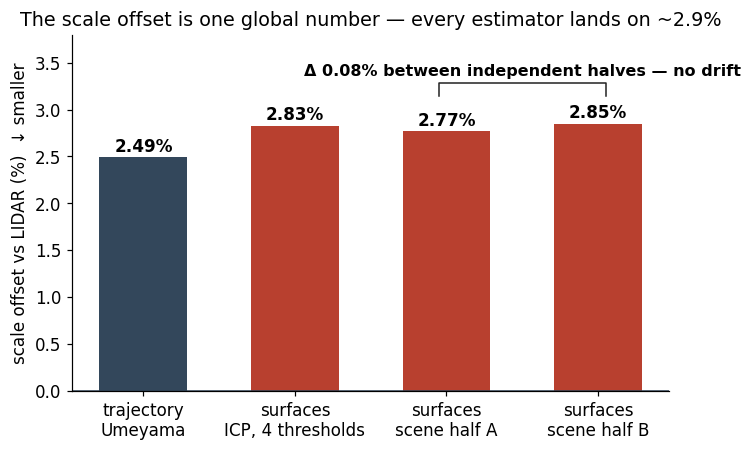
Ignoring the offset is not an option, and not only for the tape-measure test: locking scale to 1 degrades the whole accuracy table — the geometry gets blamed for what is really a gauge error.
| Alignment | median | p90 | within 5 cm |
|---|---|---|---|
| rigid only — scale locked to 1 | 5.9 cm | 41.9 cm | 44.9% |
| with the measured scale correction | 3.9 cm | 27.3 cm | 59.5% |
A 2.9% scale error costing 2 cm of median accuracy is the whole story of this section in one row: the residual error budget of this reconstruction is so small that a scale gauge most surveys would shrug at is the dominant term. So — where does the 2.9% come from? Two suspects: the reconstruction accumulated it along the walk, or it inherited it from somewhere. The next two sections interrogate them in turn.
05Ruling out drift
It is one global gauge factor, not error accumulating along the path
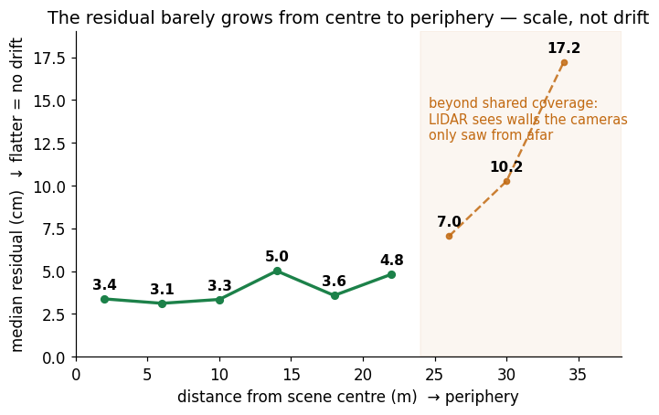
The tempting story is the classic one: image-based surveys drift, error compounds with distance, and 118 m is a long walk. We nearly wrote that sentence. It is wrong, and the scene itself proves it. If error accumulated along the path, two independent halves of the scene would disagree about scale, and the residual would grow toward the periphery. Neither happens: the two halves return the same scale to within 0.08%, and the median residual moves only from 3.2 cm at the scene centre to 5.5 cm at the periphery.
The same effect explains the long tail of the headline distribution, and it is worth seeing where those «bad» points actually live. Painting every reconstructed point by its measured distance to the LIDAR puts the red exactly where the geometry argument says it should be — distant façades and vegetation at the edge of coverage, not the surveyed core:
06The verdict on the 2.9%
The reconstruction did not create the 2.9% — and it can prove it
With drift ruled out, the remaining suspect is the pipeline's source of absolute scale. Our reconstructions are made metric by the AR poses of mobile-device photos captured alongside the 360° walk [4] — 95 of them in this scene. That gives us a decisive experiment: compare the finished model against its own reference. If the reconstruction distorted scale, it would disagree with the very poses it was scaled from.
It does not. The model reproduces its AR reference to 0.03% in scale and 1.2 cm median in position (p90 2.7 cm). The reconstruction is a faithful copy of the gauge it was handed; the 2.9% is a disagreement between the gauge and the LIDAR, passed through intact.
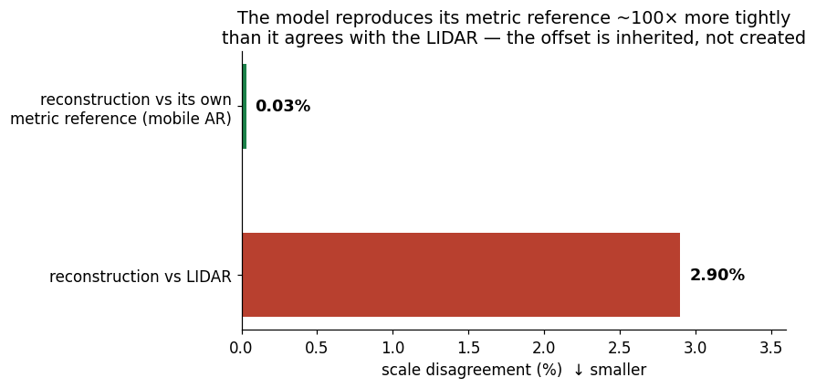
Two structural observations turn this from an excuse into a roadmap. First, the device: the reference photos were taken with an iPhone 15 without a LiDAR sensor, on purpose — that is the median device of our users, and we wanted the validation to reflect a typical capture, not a best-case one. Its ARKit scale comes from visual-inertial odometry alone, exactly the quantity a phone LiDAR helps pin down, so a gauge error of a few percent is unsurprising — and repeating the capture with a LiDAR-equipped phone is the obvious next measurement. Second, the coverage: the 95 reference photos span roughly 6 × 5.7 m of a 40 × 25 m site, so global scale is extrapolated from under 4% of the surveyed area, and any local bias in the AR poses there propagates to the whole model. Both levers — a better reference device and wider reference coverage — are capture-time fixes that require no change to the reconstruction itself.
And one last twist: which side of the 2.9% disagreement is actually right? The LIDAR is a consumer instrument with its own ~4 cm declared error budget [6], so «LIDAR = truth» is not granted. We ran the crudest possible third gauge: a tape measure over a row of six floor tiles on site — 201 cm in the real world, 200.5 cm over the same span in the delivered model, a −0.25% difference well within tape-and-tile tolerance. On that span the model's absolute scale is essentially right, which — given that the model copies its AR reference to 0.03% — hints that a good share of the 2.9% may sit on the LIDAR's side of the disagreement, not ours. One hand-taped span at one location decides nothing at percent level across a 40 m scene; read it as directional. But it is the difference between «our model is 2.9% too large» and the more honest «our model and the LIDAR disagree by 2.9%, and the only tape measure on record votes for the model».
07A blind check
The alignment recovers rig geometry it was never told
Every number so far rests on one alignment, so the alignment deserves its own audit — ideally against a quantity it could not have optimized for. The rig provides one: the LIDAR rode about 70 cm below the 360° camera on the same pole. The cloud-to-cloud alignment was computed from surface correspondences alone; it knows nothing about hardware. Yet measuring both camera heights above the LIDAR's floor plane in the aligned frame returns 2.15 m and 1.45 m — a recovered offset of 69.8 cm.
| Quantity | measured from the aligned clouds |
|---|---|
| 360° camera height above LIDAR floor | 2.15 m |
| LIDAR sensor height above LIDAR floor | 1.45 m |
| recovered vertical rig offset (physical: ~70 cm) | 69.8 cm |
Two honest footnotes. First, «~70 cm» is a tape-measure figure for the physical rig, so read the last millimetres of that agreement as luck; the point is that a blind geometric estimate lands on the hardware to well under the error budget it is auditing. Second, the trajectory figure of §02 uses the report's trajectory-alignment protocol; our recomputation for this note, which reuses the cloud alignment instead, gives an even smaller 3.4 cm median — we quote the larger published number and treat the difference as protocol sensitivity, not accuracy gained.
Below, the full evidence in one place: both clouds, both trajectories — the two paths ride visibly ~70 cm apart, as the rig dictates — and the measured per-point error as a toggleable layer. The claim of this note is that green and gray are the same site to about four centimetres; here you can check it.
| Surface agreement (after scale correction) | median | p68 | p90 | within 5 cm | within 10 cm |
|---|---|---|---|---|---|
| published table (2026-07-28) | 3.9 cm | 6.6 cm | 27.3 cm | 59.5% | 77.6% |
| recomputed for this note from the archived clouds | 3.9 cm | 6.7 cm | 28.1 cm | 59.2% | 77.1% |
08Why it matters
Relative accuracy is the hard part — and that part is done
A reconstruction error has two very different components. The shape error — walls in the wrong place, surfaces warped, loops that do not close — is structural: no post-processing removes it, and it is where image-based methods historically lose to LIDAR over long paths. The gauge error — everything uniformly 2.9% large — is one number, fully characterised, constant across the scene, and removable by a single multiplication the moment any trusted distance is known.
This study says our pipeline's error is almost entirely of the second kind. Shape agreement with a LIDAR that shares none of our assumptions: 3.9 cm median across a 40 m scene, drift-free to 0.08% over a 118 m walk, from a ten-minute single-operator capture — against a survey instrument on a tripod-free run of the same duration. And the gauge chain is not a black box: the model provably copies its reference to 0.03%, so improving absolute scale is a data-collection task (wider reference coverage), not a research risk.
The equally practical corollary: do not buy accuracy claims without an independent instrument. Had we validated the pipeline against its own metric reference — the natural in-house test — we would have reported 0.03% scale and 1.2 cm residuals and gone home happy, blind to a 2.9% offset that only an instrument outside our stack could reveal.
Methods note
Protocol. Both reconstructions come from one capture session on a shared rig (LIDAR ~70 cm below the 360° camera). Alignment: closed-form Umeyama similarity over arc-length trajectory correspondences (searched over travel direction and trim), then scaled ICP on the dense clouds at 50/25/12/6 cm thresholds, both clouds at a 5 cm voxel grid [2,3]. Accuracy is the distance from each of 1.07 M reconstructed points to the nearest LIDAR point at the same voxel size; trajectory agreement uses the report's trajectory alignment. Scale was cross-validated by re-estimating it independently on each half of the scene and by profiling the residual against distance from the scene centre.
Data rigor. Every headline number was recomputed for this note from the archived artifacts (aligned dense cloud, LIDAR cloud, both camera-pose sets) with an independent implementation [5]; the published table is reproduced to rounding (median 3.89 vs 3.9 cm, within-10 cm 77.1% vs 77.6%, p68 within 1 mm; the coverage-dominated p90 differs by 8 mm). Figures p1, p3 and p4, the error heatmap and the 3D viewer are built from that recomputation; the per-half and rigid-only aggregates are quoted from the published analysis, whose intermediate alignments were not archived. The p90 and the distribution tail are stated as coverage-contaminated rather than corrected, since point-level coverage labels do not exist.
Limits. One site, one session, outdoor daylight: transfer of the 3.9 cm figure to interiors, low light or larger sites is unmeasured. The LIDAR is a reference instrument, not truth — its declared accuracy (~4 cm [6]) is of the same magnitude as the agreement we measure — so read «3.9 cm» as agreement between instruments, not absolute error. The 2.9%-vs-LIDAR attribution to the AR reference is an inference from the 0.03% model-to-reference agreement; arbitrating it properly needs surveyed targets. The only third gauge on record is the hand-taped six-tile span of §06 (201 vs 200.5 cm): it favors the model's gauge but is a single ~2 m measurement at one location, directional only. The reference device was deliberately a non-LiDAR iPhone 15 (median-user hardware): the 2.9% characterises that device class, and both better hardware and wider reference coverage remain unmeasured levers. Nearest-point distances at a 5 cm voxel slightly overstate true surface distance everywhere; the effect is common to both table rows.
09Conclusions
What we take away
A single-pass 360° walkthrough reproduces a simultaneous LIDAR survey to 3.9 cm median over a 40 m scene, with three quarters of the surface within 10 cm and no measurable drift along 118 m — and its one systematic discrepancy is a uniform, fully characterised 2.9% scale disagreement with the LIDAR that the geometry provably did not create: it lives in the gauge chain, it is removable with a single scalar, and the one tape measurement on record suggests the model's scale may already be the closer one to the real world.
The transferable recipe is the validation itself: align trajectories closed-form (never free-scale ICP on curves), take scale from surfaces, cross-validate it on scene halves, profile the residual radially to separate gauge from drift, test the finished model against its own reference to locate blame, and keep one blind quantity — ours was the rig offset — as the audit the alignment cannot cheat.
—References
- Schönberger & Frahm. Structure-from-Motion Revisited (COLMAP). CVPR 2016 — the SfM framework underlying the pipeline's pose estimation.
- Umeyama. Least-squares estimation of transformation parameters between two point patterns. TPAMI 1991 — the closed-form similarity transform used for trajectory alignment.
- Besl & McKay. A Method for Registration of 3-D Shapes (ICP). TPAMI 1992 — basis of the scaled-ICP surface refinement.
- Apple. ARKit — visual-inertial tracking providing the mobile-AR poses that give the pipeline metric scale; the suspect this note convicts for the 2.9%.
- Zhou, Park & Koltun. Open3D: A Modern Library for 3D Data Processing. 2018 — used for the independent recomputation and the cloud renders in this note.
- 3DMakerpro. Eagle 3D LIDAR scanner (standard edition) — the reference instrument of this study; accuracy of ~4 cm per manufacturer specification (product page).
- OVER Research. lidar-validation — companion repository: the alignment script that reproduces this note's headline numbers from the two published point clouds, with the data on Google Drive (github.com/OVR-Platform/lidar-validation).